Falcon: Introduction to notebook quickstarters
Falcon is a live simulation where your model plays the role of a tracker, trying to follow the movement of a dove in flight. At every tick, you receive partial observations and must predict where the dove will be next (in HORIZON secondes).
The goal: Maximize likelihood — the score measuring how well your predicted probability distribution matches the dove’s true future positions. The higher the likelihood, the better calibrated your model.
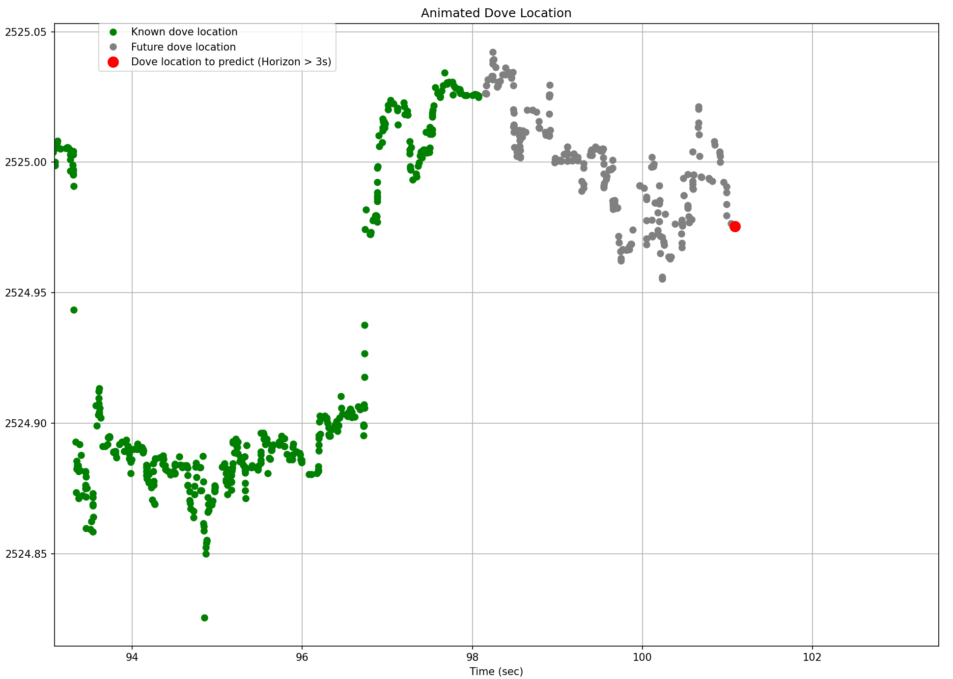
Visualize the challenge:
The following animated graph shows the dove’s true (observed) locations and the future locations on an Horizon of 3 secondes.
How the Game Works
-
You receive updates (ticks) containing the dove’s latest location.
-
Your tracker updates its internal model (
tick()). -
Then you return a probability density prediction (
predict()), not just a point estimate, representing where you believe the dove will be inHORIZONseconds.
Example output:
{
    "type": "mixture",
    "components": [
        {
        "density": {"type": "builtin", "name": "norm",
                    "params": {"loc": 3.7, "scale": 0.8}},
        "weight": 0.6
        },
        {
        "density": {"type": "builtin", "name": "cauchy",
                    "params": {"loc": 3.5, "scale": 1.2}},
        "weight": 0.4
        }
    ]
}
The leaderboard evaluates log-likelihood of your predicted distribution against real dove locations, so both accuracy and uncertainty estimation matter.
Live graph example (3 secondes Horizon):
You can explore all available distributions in the densitypdf package.
-
Dataset Description: Learn the data structure
-
Game Rules: Understand how the game works and scoring
-
Probabilistic forecasting: Explanation of probabilistic forecasting
Probabilistic forecasting can be handled through various approaches, including:
- Variance forecasters
- Quantile forecasters
- Interval forecasters
- Distribution forecasters
Quickstarters: From Baselines to Smarter Trackers
Now that you understand the game mechanics, let’s explore some ready-to-use quickstarter trackers.
These templates will help you get started quickly with probabilistic forecasting and test ideas.
1. Naive Tracker
The NaiveTracker is the simplest strategy — it predicts that the dove will stay near its last observed location.
This tracker does not learn from past data, but it’s perfect for testing your setup and understanding the prediction interface. It uses the most recent observation as the mean of a Gaussian distribution and the scale (uncertainty) is fixed:
from birdgame.trackers.trackerbase import TrackerBase
from birdgame import HORIZON

class NaiveTracker(TrackerBase):
    def __init__(self, horizon=HORIZON):
        super().__init__(horizon)
        self.current_x = None

    def tick(self, payload, performance_metrics=None):
        self.current_x = payload['dove_location']
        t = payload["time"]

    def predict(self):
        return {
            "type": "mixture",
            "components": [{
                "density": {"type": "builtin", "name": "norm",
                     "params": {"loc": self.current_x, "scale": 0.01}},
                "weight": 1
            }]
        }
This code is sufficient for submission to the challenge. A class that inherits from
TrackerBase, processes the payload intick()and returns a probability density prediction inpredict().You just need to copy it into a notebook and submit it on the Falcon submit a notebook section. You can also copy it into a python file and submit it on the Falcon submit files section
2. EWMA Variance and Mixture of Gaussians (variance forecaster)
Full quickstarter notebook: EWMA Variance Tracker
A method for tracking variance over time while giving more importance to recent observations using an exponential decay factor.
The EMWAVarTracker fits a mixture of two Gaussian distributions to model both typical fluctuations and extreme moves.:
-
Core distribution — captures regular variance
-
Tail distribution — captures extreme deviations
It uses EWMA (Exponentially Weighted Moving Average) to update variance dynamically.
Minimal example:
from birdgame.stats.fewvar import FEWVar

class EMWAVarTracker(TrackerBase):
    def __init__(self, horizon=HORIZON):
        super().__init__(horizon)
        self.current_x = None
        self.ewa_dx_core = FEWVar(fading_factor=0.0001)
        self.ewa_dx_tail = FEWVar(fading_factor=0.0001)

    def tick(self, payload, performance_metrics=None):
        x = payload['dove_location']
        # Adds a new value to the quarantine list.
        # The value will become available for prediction processing
        # at `time + self.horizon`.
        self.add_to_quarantine(payload['time'], x)
        # Returns the most recent valid data point from quarantine,
        # if available.
        prev_x = self.pop_from_quarantine(payload['time'])
        if prev_x is not None:
            self.ewa_dx_core.update(np.clip(x-prev_x, -2, 2))
            self.ewa_dx_tail.update(2*(x-prev_x))
        self.current_x = x

    def predict(self):
        if self.ewa_dx_core.get() == 0.0:
            return None # warmup period
        return {
            "type": "mixture",
            "components": [
                {"density": {"type": "builtin", "name": "norm",
    "params": {"loc": self.current_x,
             "scale": math.sqrt(self.ewa_dx_core.get())}},
    "weight": 0.95},
                {"density": {"type": "builtin", "name": "norm",
    "params": {"loc": self.current_x,
             "scale": math.sqrt(self.ewa_dx_tail.get())}},
    "weight": 0.05}
            ]
        }
You can return
Noneduring your tracker’s warmup period — no wealth is at stake during this time.
3. Online Quantile Linear Regression (quantile forecaster)
Full quickstarter notebook: Quantile Linear Regression
The QuantileRegressionRiverTracker uses online quantile regression to track the dove location. Quantile forecasting enables the creation of prediction intervals by estimating lower and upper quantiles.
Minimal example:
from river import linear_model, preprocessing, optim

class QuantileRegressionRiverTracker(TrackerBase):
    def __init__(self, horizon=HORIZON):
        super().__init__(horizon)
        self.current_x = None
        self.models = {}
        for alpha in [0.05, 0.5, 0.95]:
            scale = preprocessing.StandardScaler()
            learn = linear_model.LinearRegression(
                intercept_lr=0,
                optimizer=optim.SGD(0.005),
                loss=optim.losses.Quantile(alpha=alpha)
            )
            model = scale | learn
            model = preprocessing.TargetStandardScaler(regressor=model)
            self.models[f"q {alpha:.2f}"] = model

    def tick(self, payload, performance_metrics=None):
        x = payload['dove_location']
        self.add_to_quarantine(payload['time'], x)
        prev_x = self.pop_from_quarantine(payload['time'])
        if prev_x is not None:
            for m in self.models.values():
                m.learn_one({"x": prev_x}, x)
        self.current_x = x

    def predict(self):
        x_mean = self.models["q 0.50"].predict_one({"x": self.current_x})
        y_lower = self.models["q 0.05"].predict_one({"x": self.current_x})
        y_upper = self.models["q 0.95"].predict_one({"x": self.current_x})
        scale = max(abs(y_upper - y_lower)/3.29, 1e-6)
        return {
            "type": "mixture",
            "components": [{"density": {"type": "builtin", "name": "norm",
             "params": {"loc": x_mean, "scale": scale}}, "weight": 1}]
        }
It predicts multiple quantiles (5%, 50%, 95%) to capture uncertainty dynamically,
with the scale computed as (y_upper - y_lower) / (norm.ppf(q_upper) - norm.ppf(q_lower)).
4. Automatic Exponential Smoothing (variance forecaster)
Full quickstarter notebook: AutoETS
AutoETS (Auto Exponential Smoothing) from sktime is an automatic forecasting method that applies exponential smoothing to time series data with trend and seasonality.
Minimal example:
from sktime.forecasting.ets import AutoETS

class AutoETSsktimeTracker(TrackerBase):
    def __init__(self, horizon=HORIZON):
        super().__init__(horizon)
        self.current_x = None
        self.last_observed_data = []
        self.forecaster = AutoETS(auto=True, sp=1,
                                  information_criterion="aic")
        self.scale = 1e-6
        self.num_data_points_max = 5
        self.prev_t = 0

    def tick(self, payload, performance_metrics=None):
        x = payload["dove_location"]
        t = payload["time"]
        self.current_x = x

        # Collect and process observations only at horizon-based intervals
        if t > self.prev_t + self.horizon:
            self.last_observed_data.append(x)
            self.prev_t = t
            if len(self.last_observed_data) >= self.num_data_points_max:
                y = np.array(
                      self.last_observed_data[-self.num_data_points_max:]
                     )
                self.forecaster.fit(y)
                var = self.forecaster.predict_var(fh=[1])
                self.scale = np.sqrt(var.values.flatten()[-1])

                # Update last observed data (to limit memory usage
                # as it will be run on continuous live data)
                self.last_observed_data = self.last_observed_data[-
                                          (self.num_data_points_max + 2):]

    def predict(self):
        if len(self.last_observed_data) < self.num_data_points_max:
            return None  # warmup period
        return {
            "type": "mixture",
            "components": [{"density": {"type": "builtin", "name": "norm",
              "params": {"loc": self.current_x, "scale": self.scale}},
              "weight": 1}]
        }
Performance tip: Inference must be completed in under 50 ms.
In the quickstarter notebook, you will find an example of asynchronous retraining to avoid blocking predictions while updating the model in the background.Memory tip: The tracker keeps only the most recent observations to limit memory usage, which is important for continuous live data streams.
5. Natural Gradient Boosted (distribution forecaster)
Full quickstarter notebook: NGBoost
NGBoost (Natural Gradient Boosting) is a method for probabilistic regression that extends gradient boosting to predict full probability distributions instead of just point estimates. It predicts a Gaussian distribution, capturing both mean and uncertainty:
-
introduction: https://stanfordmlgroup.github.io/projects/ngboost/
-
user guide: https://stanfordmlgroup.github.io/ngboost/intro.html
-
guide to add new distribution target and scoring: https://stanfordmlgroup.github.io/ngboost/5-dev.html
6. Run the Wealth Distribution Simulation with Multiple Trackers
Full quickstarter notebook: Wealth Distribution
A notebook is available to simulate the Falcon Wealth Game using multiple trackers at once.
This simulation allows you to observe how different prediction models interact under shared conditions, competing for the same reward pot based on their likelihood performance.
Each tracker receives an initial wealth allocation and invests a small fraction of it at every tick.
The reward pot is then redistributed proportionally to each model’s likelihood score, reflecting both predictive accuracy and model diversity.
You can easily include any tracker (e.g:EMWAVarTracker, AutoETSsktimeTracker, NGBoostTracker, QuantileRegressionRiverTracker) and watch how wealth evolves over time.
Wealth distribution simulation on 3 trackers:
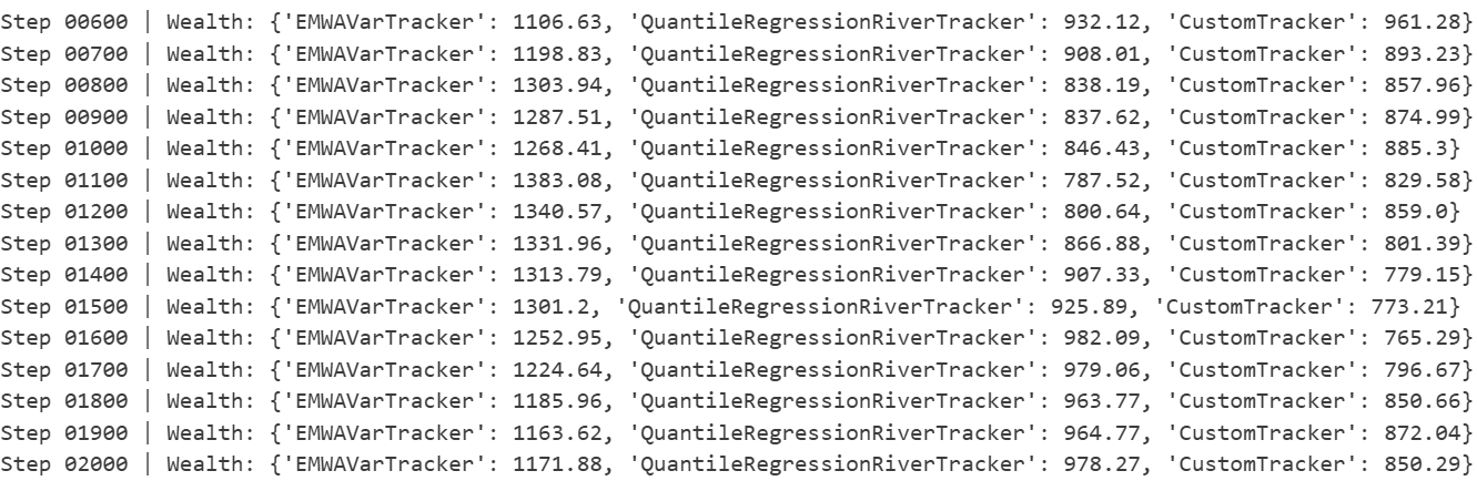
NOTE:
At every tick, you receive the dove’s current location along with additional information:
{'time': 53952.14900016785, 'falcon_location': 2200.15, 'dove_location': 2200.16, 'falcon_id': 72, 'falcon_wingspan': 0.2014}
This graph shows the dove’s known location along with multiple falcon IDs:
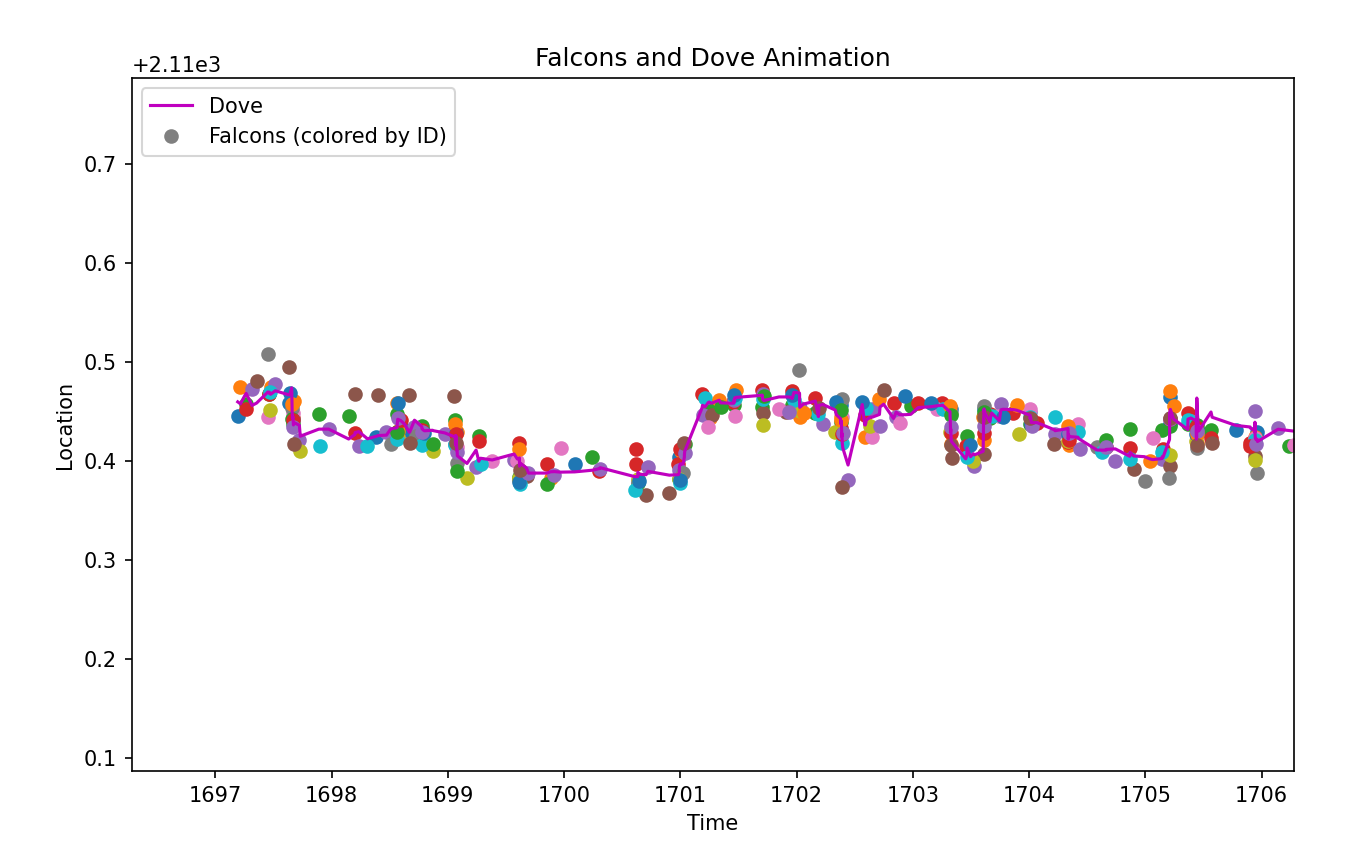
The falcon locations are shown as colored dots on the figure above. Some falcons may provide useful information as to (track) the future location of the dove, or the uncertainty of the same, whereas others may not. Their utility, or otherwise, is for you to determine.
 Submitting Your Tracker to the Falcon CrunchDAO Platform
Once you’ve explored or customized one of the Quickstarter notebooks, submitting your tracker is straightforward.
-
Open a Quickstarter Notebook
Choose one of the ready-to-run notebooks such as:
-
Customize (Optional)
You can adjust:-
Model parameters
-
Update logic inside
tick() -
Uncertainty estimation inside
predict()
Just make sure your tracker class inherits from
TrackerBaseand defines both methods correctly. -
-
Submit to the Platform
Go to the Falcon Submission Page, upload your notebook and click Submit.
You can also check the documentation.
Your tracker will then compete live in the Birdgame simulation, with real-time log-likelihood scores displayed on the leaderboard.